p-adic Landscapes

Experiments on neighbour-hyperplane graphs for ultrametric ($p$-adic) linear regression: basins of attraction, local minima networks, and barriers on a finite model space obtained by interpolating $d{+}1$ points.

Links

Repo scripts: see code/padic_linear_regression.py and code/make_experiment_report.py.

Baseline noisy policy comparison

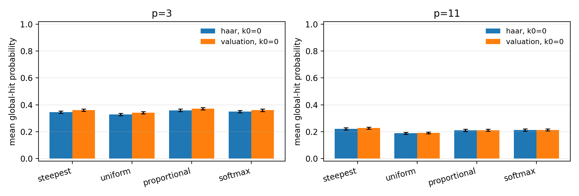
Multi-policy comparison at baseline noise (k0=0), for p=3 and p=11.

Global-hit probability vs noise

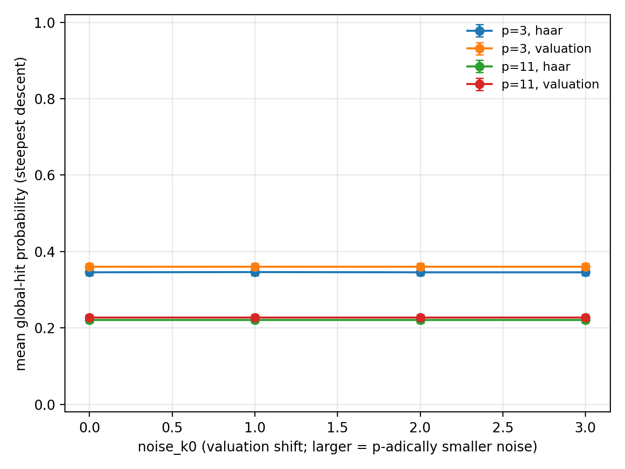
Steepest-descent global-hit probability as noise decreases (larger k0).

P(true beta is globally optimal) vs noise

Probability true beta is globally optimal vs noise

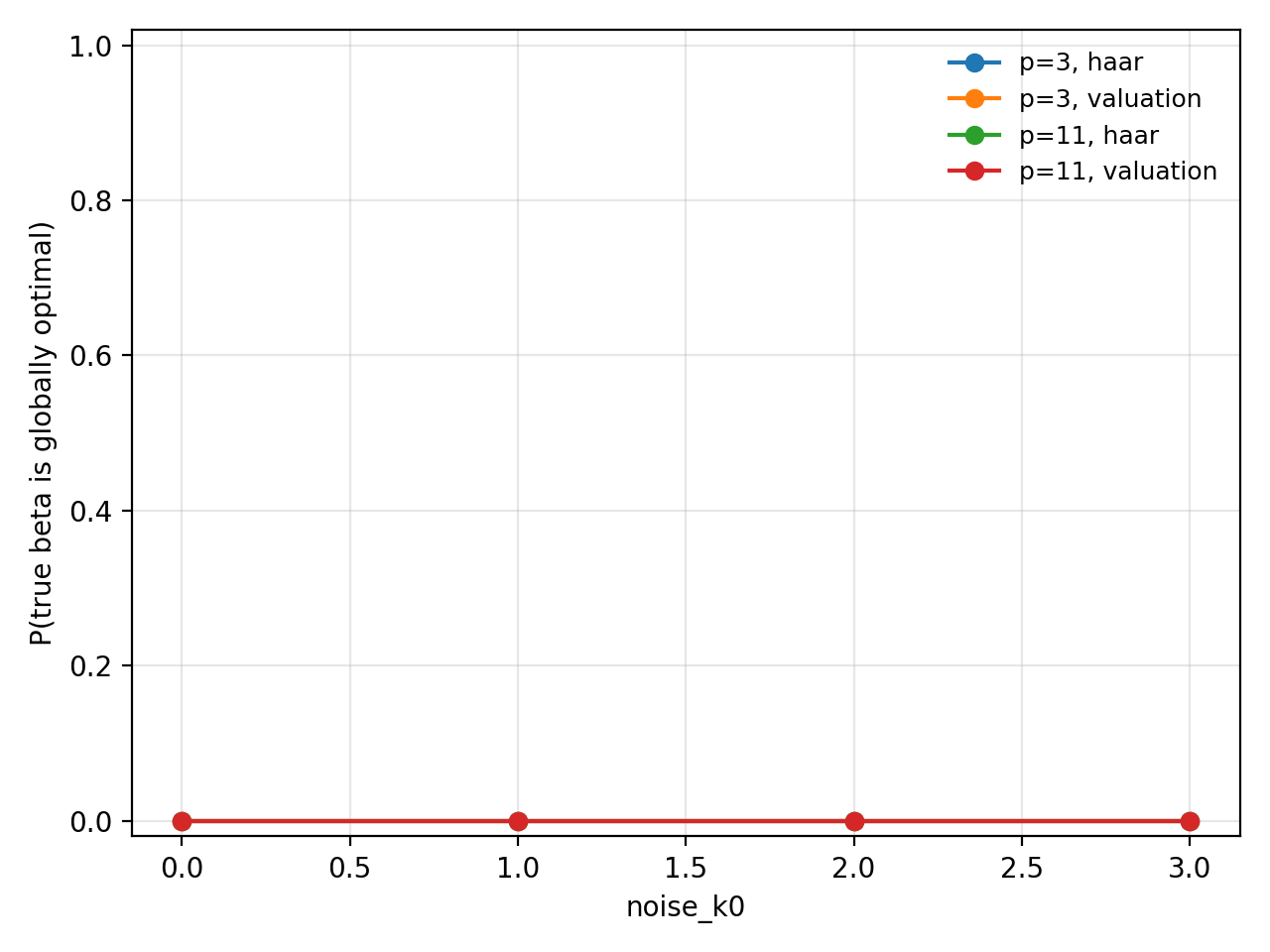
How often the ground-truth coefficients are globally optimal under the loss.

Dimension/noise trend heatmap

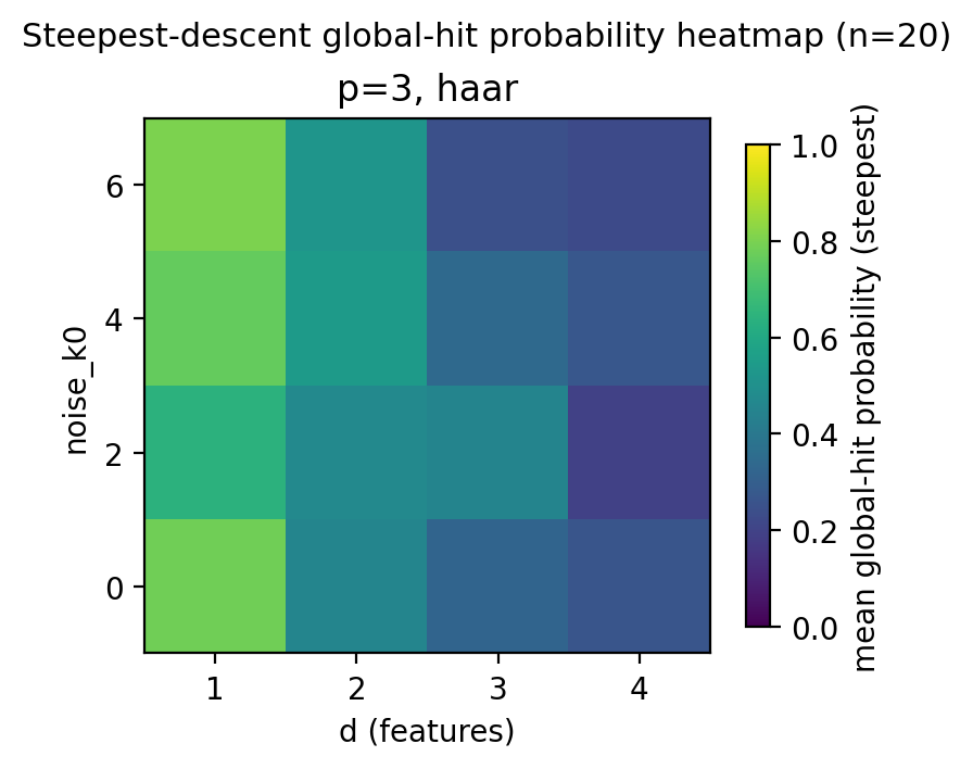
Global-hit probability heatmap across d and noise

Example sweep across dimensions d and noise levels k0 (steepest descent; n=20).

Local optima network

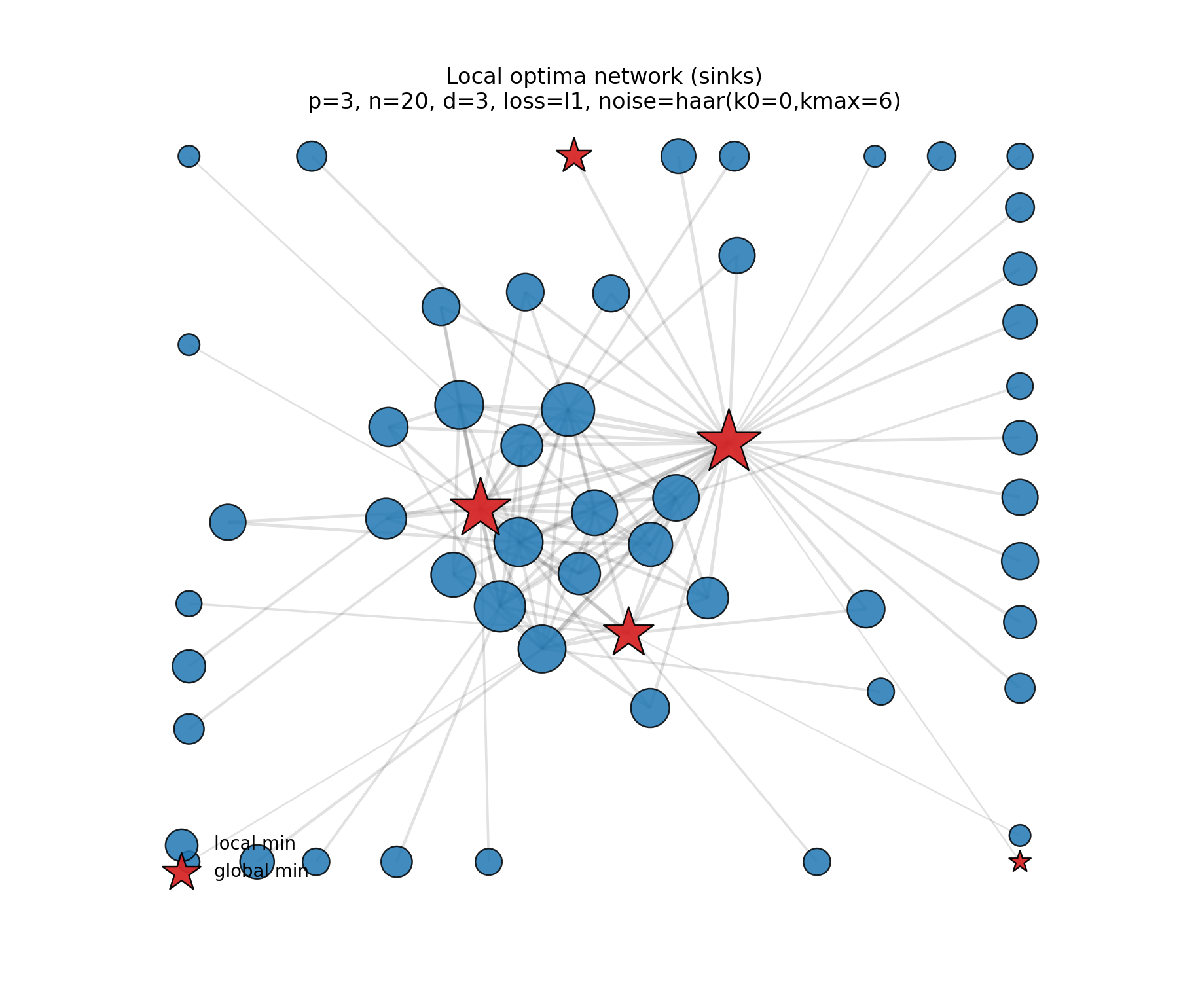
Network of local minima (node size ∝ basin size). Edges are a sparse selection of basin-boundary connections (strongest overall plus each node’s strongest edge); global minima are highlighted in red.

Local optima network backbone (MST)

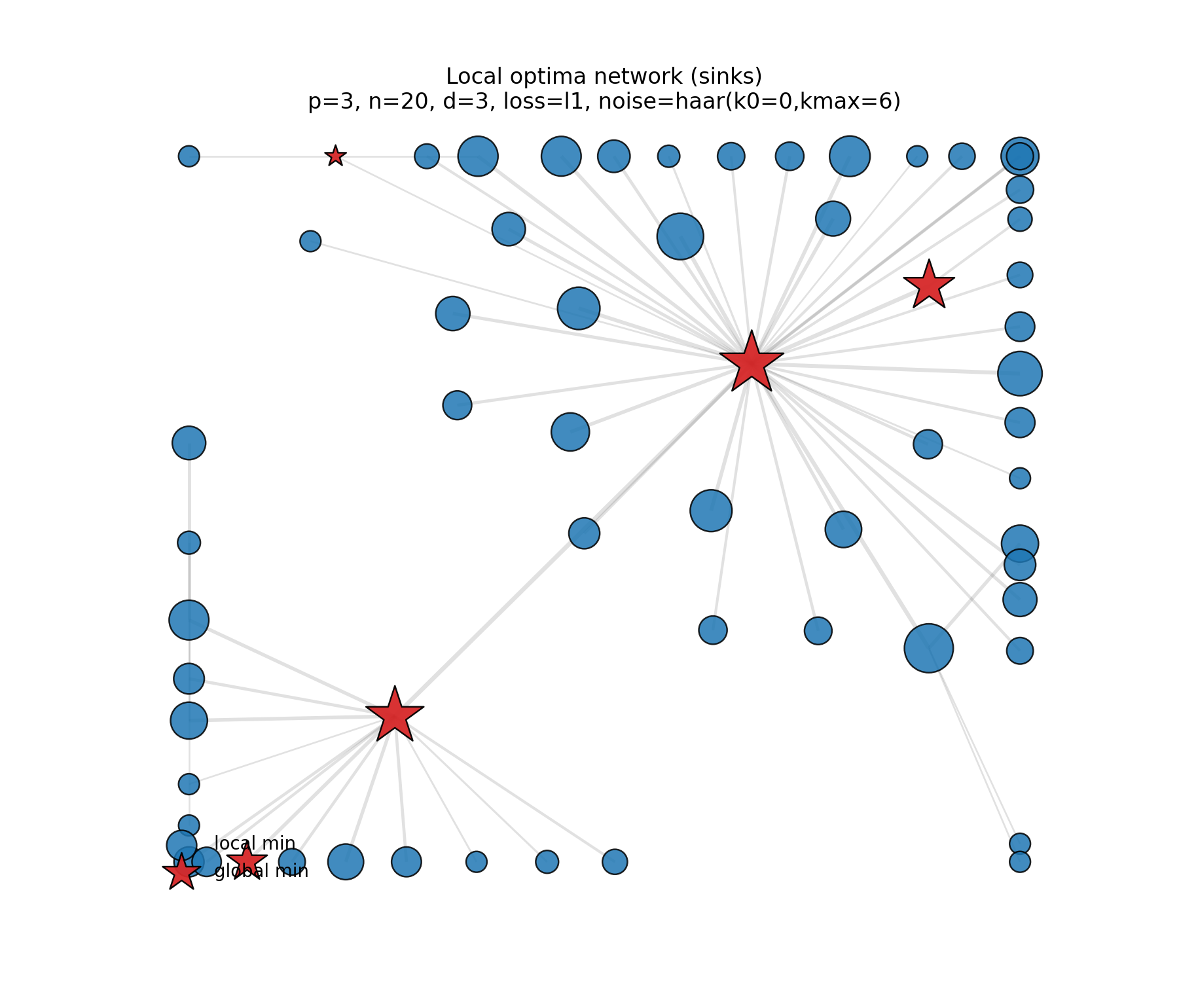
Local optima network backbone (maximum spanning tree)

Maximum spanning tree backbone of the sink network (edge weights = basin-boundary size). This gives a coarse, readable “geography” of the main basins without the wet-spaghetti effect.

Disconnectivity tree (merge tree)

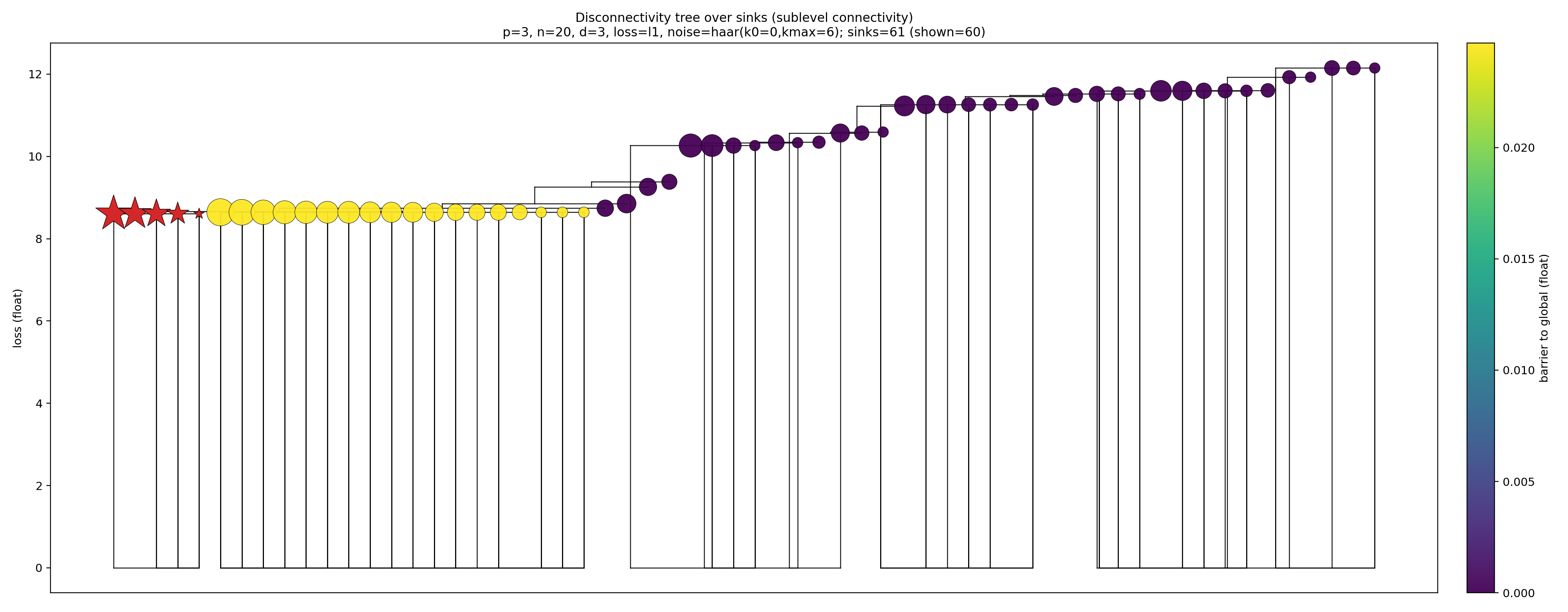
Disconnectivity tree over local minima: leaves are sinks (marker size ∝ basin size; global minima are red stars), and internal merges occur at the loss threshold where basins first become connected in the sublevel set. Leaf colour shows the barrier-to-global (minimised max-loss along a path to any global basin).

Support co-occurrence (global minima)

Support co-occurrence network (global minima)

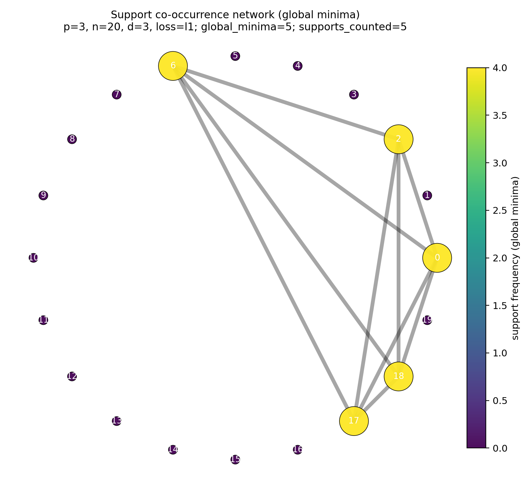
Points as nodes; edge weight counts how often a pair co-occurs in defining supports of global minima. This makes “kingmaker” points and cliques visible.

Tiny descent graph (n=5)

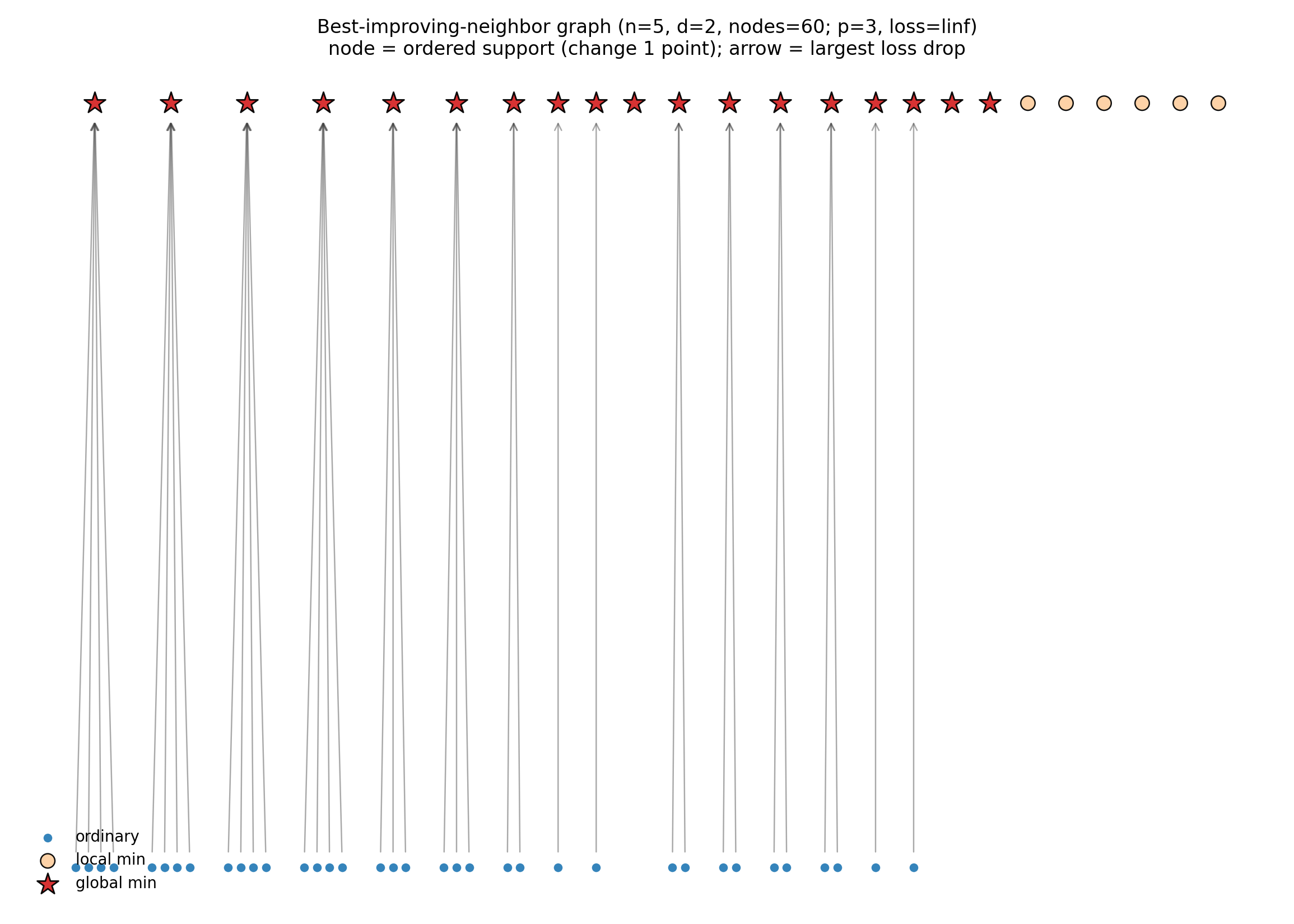
Full 60-node example (ordered triples of 3 points). Arrow from each node goes to the neighbor with the largest loss drop; global minima are stars and local minima have no outgoing arrows.

Rafting basins (n=8)

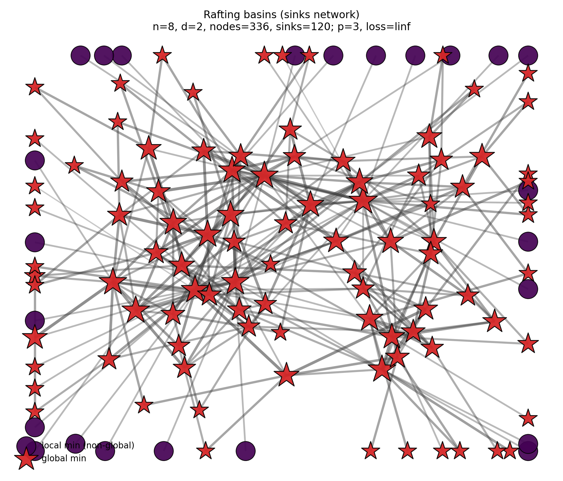
Collapse the full ordered-support graph into basins (nodes = sinks). Node size ∝ basin size; global minima are red stars; other sinks are coloured by “swim distance” (fewest one-point changes needed to reach any node in a global basin).

Swim distance histogram (n=8)

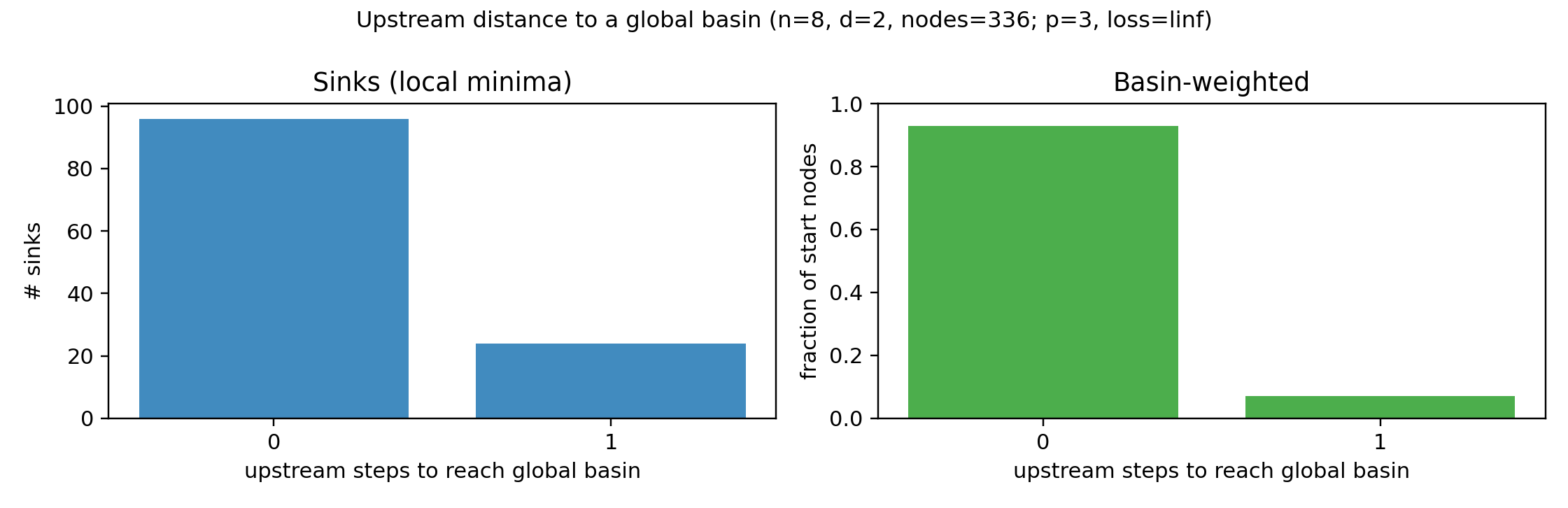
Histogram of upstream swim distance to global basin (n=8)

Distribution of swim distances: left counts sinks (local minima), right weights by basin size (fraction of starting nodes that raft to each sink).